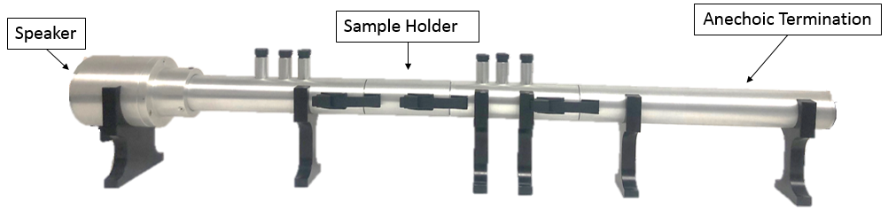
Figure 5: Complete assembled impedance tube for transmission loss testing. Speaker (left) subjects sample (contained in middle) to broadband noise to determine acoustic properties.
Next the microphones can be inserted into the tube.
2. 2 Inserting Microphones
The microphones must be inserted at the proper height into the tube. There will be two microphones on each side of the sample.
Depending on the tube design, there may be three microphone holders on each side of the sample:
- Outer Microphone Positions: By using the outer two microphone holders (65 mm distance on the Mecanum tube), the useable frequency range is 50 Hz to 2400 Hz.
- Smallest Microphone Spacing: By using the inner two microphone holders (29 mm distance on the Mecanum tube), the useable frequency range is 119 Hz to 5700 Hz.
- Unused Microphone Holder: The unused microphone holder will be sealed off with a white dummy microphone stick. There should be at least one microphone holder on each side that is not occupied.
To start, insert the microphone through the black collet as shown in Figure 5. Place the microphone all the way down into the tube until it cannot go further.
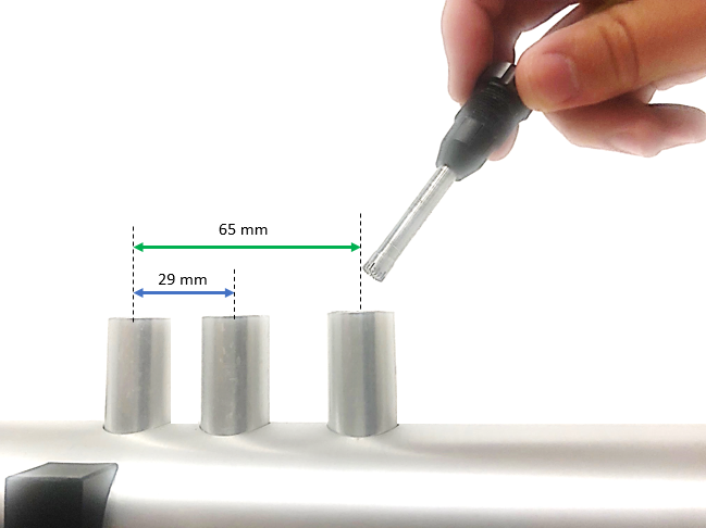
Figure 6: After inserting the microphone through the black collet holder, put the microphone into the tube until it stops.
After the microphone will not travel further, tighten the collet around the microphone as shown in Figure 7.
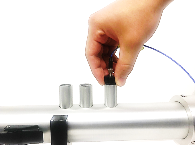
Figure 7: After pushing the microphone into the tube, thread the black collet around the microphone to secure it.
Thread the black collet to until it holds the microphone firmly in place. Note that the collet will still have exposed threads after securing the microphone.
A guide for how the microphone should be sitting in the holder is shown in Figure 8.
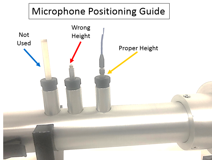
Figure 8: Microphone holder not used should be secured with white dummy plug (left), microphone not pushed until stopped at incorrect height (middle), and microphone installed properly (right).
In any impedance tube, the microphones ends are intended to be flush with the inner tube walls as shown in Figure 9.
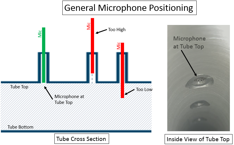
Figure 9: Microphone should be flush with top of the tube.
After the tube is assembled, the complete system should be wired as shown in Figure 10.
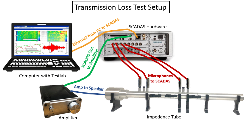
Figure 10: Connections between different components of Transmission Loss Test setup. For the initial phase calibration, the anechoic termination should be used (pictured).
Some cabling guidance (Figure 11):
- The four microphones should be plugged into the first four channels of the Simcenter SCADAS. The first microphone is closest to the speaker end of the tube.
- The DAC output of the SCADAS has an adaptor to BNC. The BNC is converted to RCA to plug into the back of the amplifier.
- The amplifier output is sent to the speaker input.
Figure 11: Cable connections of amplifier, speaker input.
Initially, the gain should be turned down on the amplifier for the tube (Figure 12).
Figure 12: Turn the gain as low as possible initially on the amplifier (turn counter clockwise as far as possible).
Be sure to turn the SCADAS hardware on.
3. Simcenter Testlab Impedance Software
Once the hardware is setup, the software can be started and setup.
3.1 Getting Started
Choose “Start -> Programs -> Simcenter Testlab -> Testlab Acoustic -> Sound Transmission Loss Testing using Impedance Tube” as shown in Figure 13.
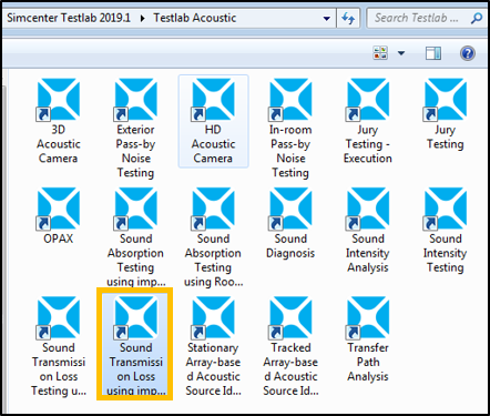
Figure 13: Start the icon labelled “Sound Transmission Loss using impedance tube”.
Using Simcenter Testlab tokens, a total of 48 tokens (and a Desktop license) are needed. The frontend driver license requires 12 tokens, and the transmission loss software requires 36 tokens.
After the software starts, choose “File -> Save As…” to store into a project file.
3.2 Channel Setup
In the Channel Setup, there should be four microphones active as shown in Figure 14. The first microphone (labelled MicA) should correspond to the microphone closest to the speaker end of the tube.
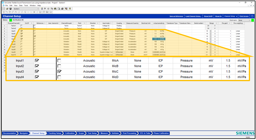
Figure 14: Channel Setup of Transmission Loss software.
put small box before zoom box
Moving away from the speaker, the microphones should be MicA, MicB, MicC, and MicD in that order. MicC should be marked as the reference.
The input mode of the microphones should be ICP unless the microphones being used required 200V polarization.
The correct sensitivity values for the microphones should be entered in the "Actual Sensitivity" field.
Before measuring, a microphone calibration should be performed. See the Knowledge base article “Simcenter Testlab: Calibration”.
3.3 Source Setup
Go to the Scope worksheet. Make sure that under “Tools -> Add-ins” the Source Control add-in is turned on. Change the source settings on the right side of the worksheet as shown in Figure 15.
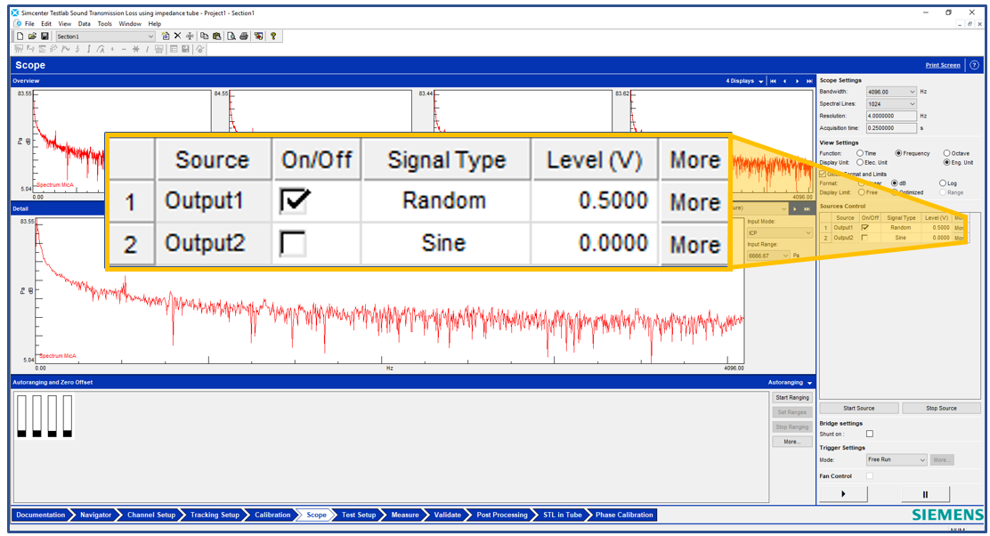
Figure 15: Source settings are located on the right side of the Scope workbook.
Make sure the source signal type is Random, and the voltage is higher than zero. For example, it can be set to 0.5 volts.
After pressing the “Start Source” button on the middle right side of the screen, adjust the amplifier gain until the interior noise levels of the tube reach 100 dB to ensure a good signal to noise ratio.
If the channels and sources are properly setup, the next step is Phase Calibration.
3.4 Phase Calibration
In this worksheet, and phase discrepancies in the measurement chain (wires, microphones, data acquisition hardware) are measured. This removes any “noise” on the transmission loss measurement caused by the hardware rather than the test article.
The microphones will be measured in different positions in the presence of the generated broadband noise to determine the phase errors. Frequency response functions (H) will be measured between the microphones.
Click on the Phase Calibration worksheet as shown in Figure 16. The phase calibration should be done with an empty tube and anechoic termination. The anechoic termination of the tube is filled with sound absorbing material.
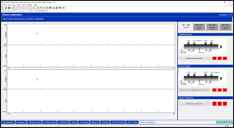
Figure 16: Phase calibration worksheet of Transmission Loss.
First click on the “Measure standard positions” button to measure the microphones in their base positions as shown in Figure 17.
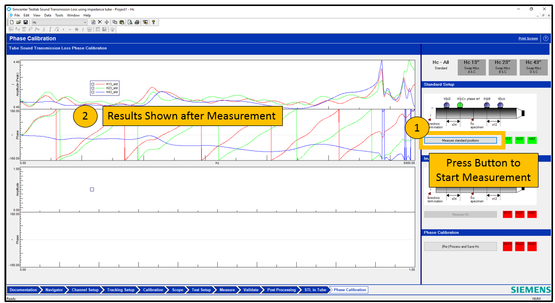
Figure 17: First measurement done in phase calibration is with microphones in standard position.
After the measurement is done, the results are shown.
Then microphones MicA and MicC must be swapped (the first microphone closest to the speaker and the third closest).
After swapping, click on the tab “Hc 13” as shown in Figure 18. Then click the measurement button “Measure 13”.
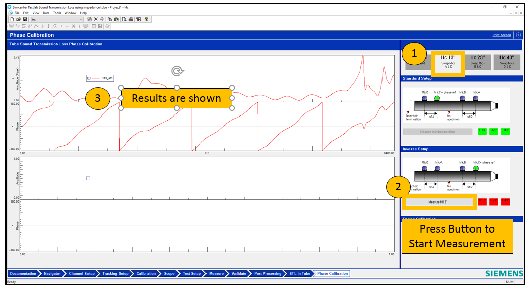
Figure 18: Second measurement (Hc 13) in phase calibration is performed with MicA and MicC swapped.
After the measurement is done, the microphones should be returned to their original position.
Then microphones MicB and MicC must be swapped (the second microphone closest to the speaker with the third closest).
After swapping, click on the tab “Hc 23” as shown in Figure 19. Then click the measurement button “Measure 23”.
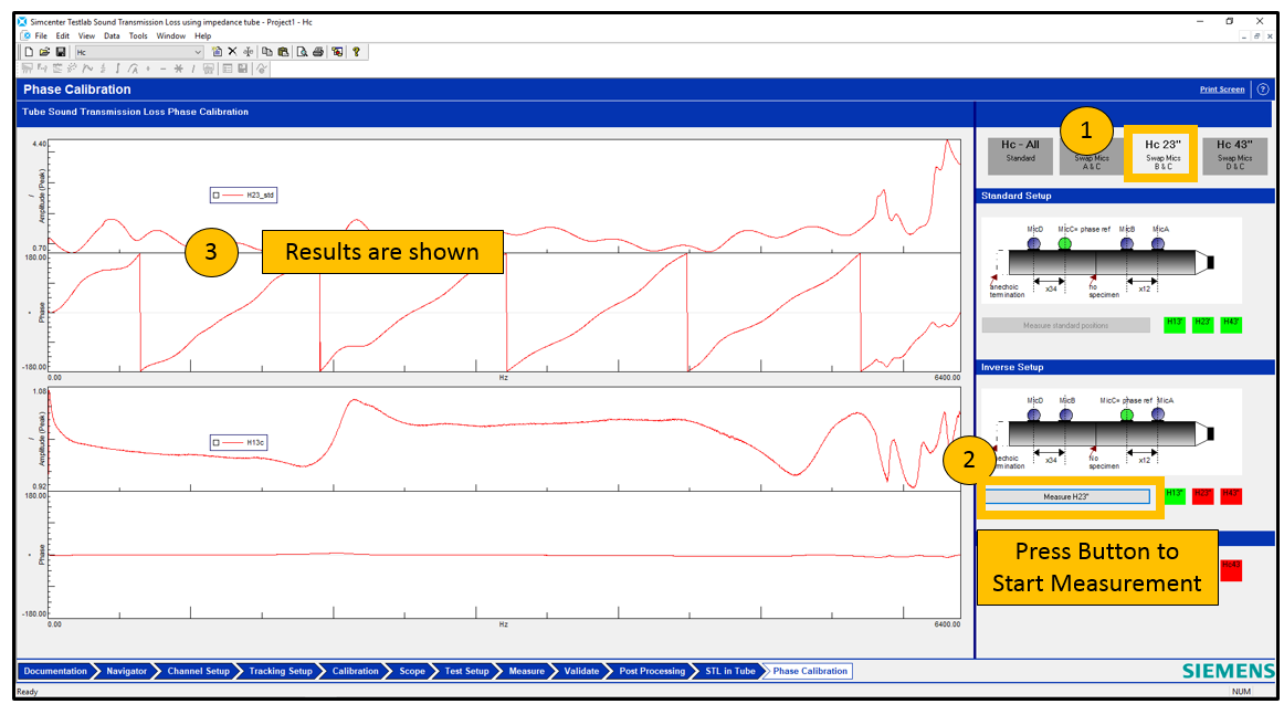
Figure 19: Third measurement (Hc 23) in phase calibration is performed with MicB and MicC swapped.
After the measurement is done, the microphones should be returned to their original position.
Then microphones MicC and MicD must be swapped (the two furthest microphones from the speaker).
After swapping, click on the tab “Hc 43” as shown in Figure 20. Then click the measurement button “Measure 43”.
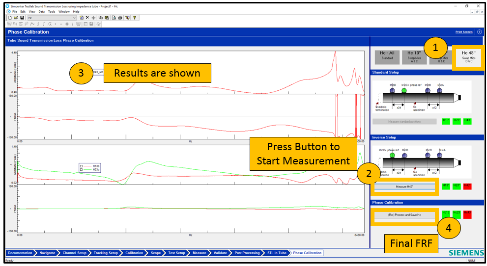
Figure 20: Fourth measurement (Hc 43) in phase calibration is performed with MicC and MicD swapped.
After the measurement is done, the microphones should be returned to their original position. Press the “Re-Process and Save Hc” button in lower right corner to finalize the phase calibration.
Now the material sample can be loaded into the tube.
3.5 Measurement
To load the sample into the tube, remove the anechoic termination. Insert the sample into one end of the sample holder as shown in Figure 21.
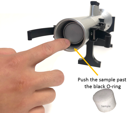
Figure 21: Push the material sample into the tube past the black O-ring.
Push the material sample past the black O-ring. The main purpose of the O-ring is to ensure there are no leaks between the two halves of the tube.
The fit of the material sample to the tube walls is critical. The sample should have been cut to exactly the tube diameter (Figure 22):
- Too Small - There should not be a gap between the sample and the wall.
- Too Big – The sample should not be so large that it is deformed or compressed when sitting in the tube.
Figure 22: Left - Sample should be cut exactly to tube diameter and not be too larger or small. Right - Sample cutter.
Some tubes will come with material cutters to ensure the sample is cut to the exact diameter of the tube.
Put the anechoic termination back in place, and then click on the “STL in Tube” worksheet.
In the upper right, enter the dimensions for the tube as shown in Figure 23. The dimensions are different depending on the tube being used. The dimensions of any tube can be entered for usage.
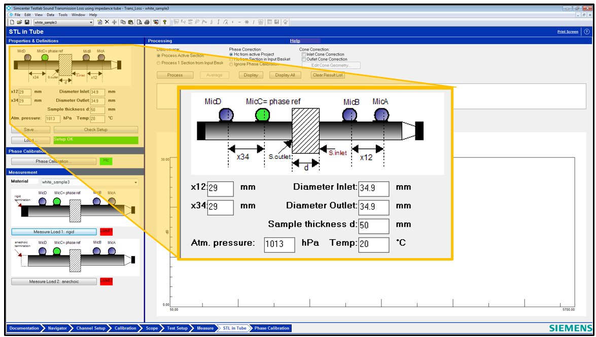
Figure 22: Set the dimensions for the tube in the upper left corner of the STL in Tube worksheet.
The following dimensions can be entered based on the tube being used:
- Mecanum Tube (MECMCICA-G): Distance (x12 and x34) between microphones 29 mm or 65 mm, diameter (inlet and outlet) is 34.9 mm.
- Spectronics Tube (SPEMCIUS-G): Distance (x12 and x34) between microphones 29.21 mm, diameter (inlet and outlet) is 34.86 mm.
- Sample Thickness: This is not used in calculating the STL. It is for later reference.
After entering the dimensions, press “Check Setup”. Phase calibration should be ON. Press the “Measure Load2 Anechoic” button in the lower left as shown in Figure 23.
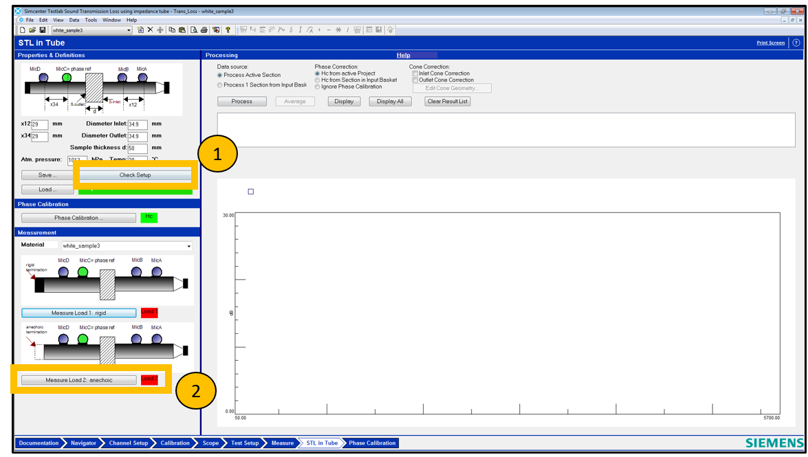
Figure 23: Measure Load2 Anechoic
After the Anechoic load measurement is done (the Load2 message should change from red to green), change out the tube to have the rigid termination as shown in Figure 24.
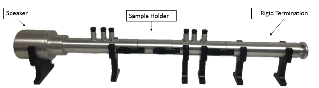
Figure 24: Impedance tube with rigid termination.
Then start the rigid measurement by pressing the button in the lower left as shown in Figure 25.
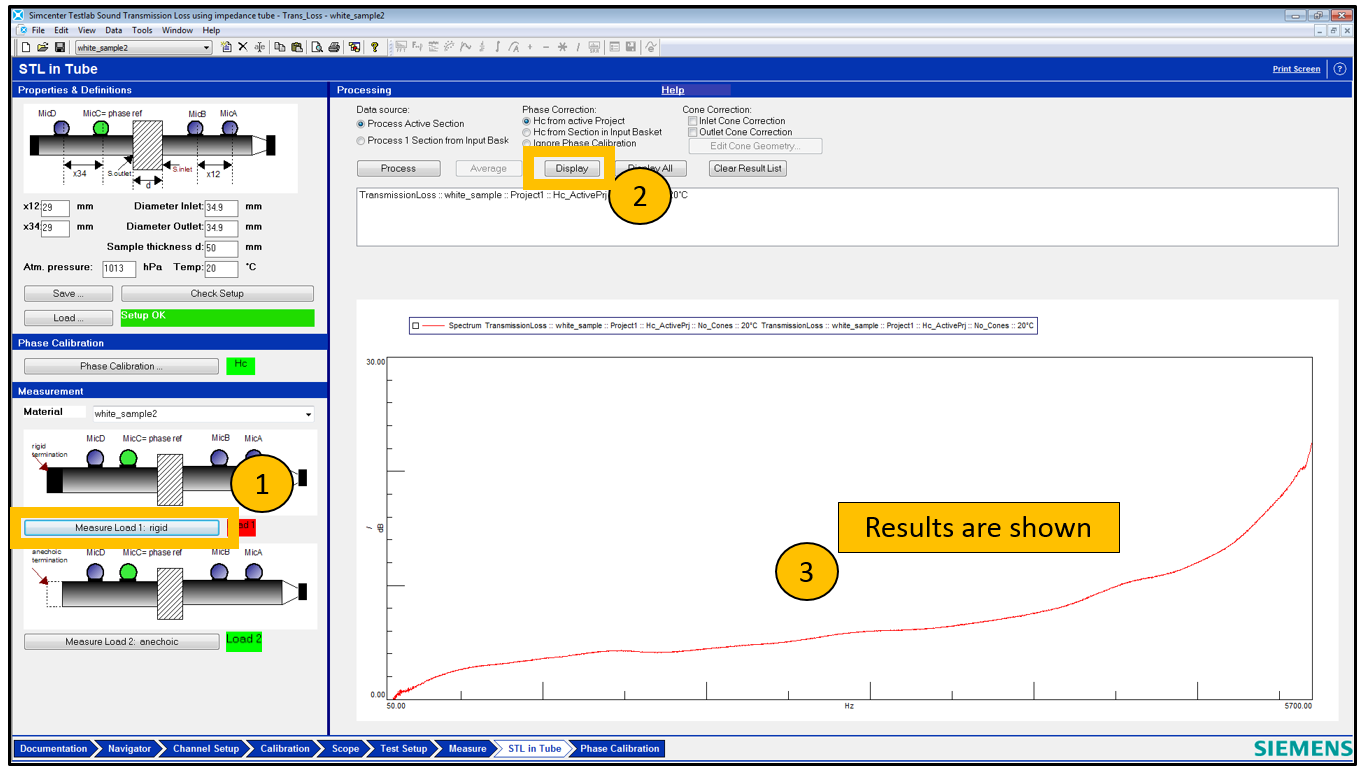
Figure 25: Measure the second load condition (rigid) and then click on the display button to view the results.
Press the “Display” button to see the results in the lower graph.
It is possible to test a different sample and overlay the results.
To do so, first enter a new “material” name in the middle left of the screen as shown in Figure 26.
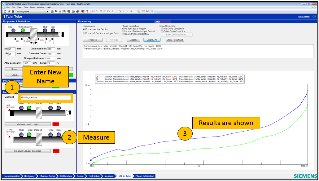
Figure 26: Enter the name for the new measurement in the middle left, and then take measurements for the second sample.
It is also possible to test items like exhausts and induction systems, not just material samples. Some considerations for doing this are shown in the next section.
4. Transmission Loss of Exhaust or Induction Systems and Cone Corrections
Transmission Loss can also be measured on parts like induction systems and exhausts as shown in Figure 27.
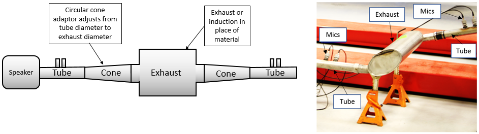
Figure 27: Left – Diagram of transmission loss setup for exhaust system. Right – Actual transmission loss test for an exhaust.
It is possible that the tube and exhaust inlet/outlet will have different diameters. In this case, conical adapters might be used to attach the exhaust and tube.
Cone adapters cause an increase in transmission loss. If cone adapters are used to test an induction or exhaust system, corrections must be made to remove this effect so that only the STL of the system of interest is calculated.
A straight pipe should have a transmission loss of 0 dB. The changing diameters of the cone adapters will create higher transmission loss than a straight pipe. A generalized example of the transmission loss created by two cone adapters is shown below (Figure 28).
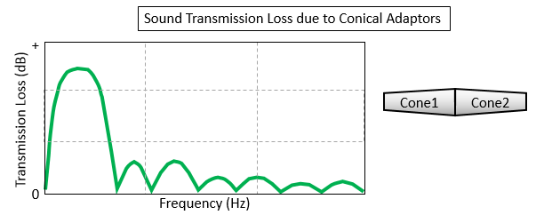
Figure 28: Using conical adaptors can cause artificial increase in the apparent transmission loss shown.
This increase in transmission loss is larger at low frequencies and follows a pattern of humps.
This increase is due to the cones, and not the exhaust system. Using the cone correction feature of Simcenter Testlab (Figure 29), this affect can be removed from the measurement.
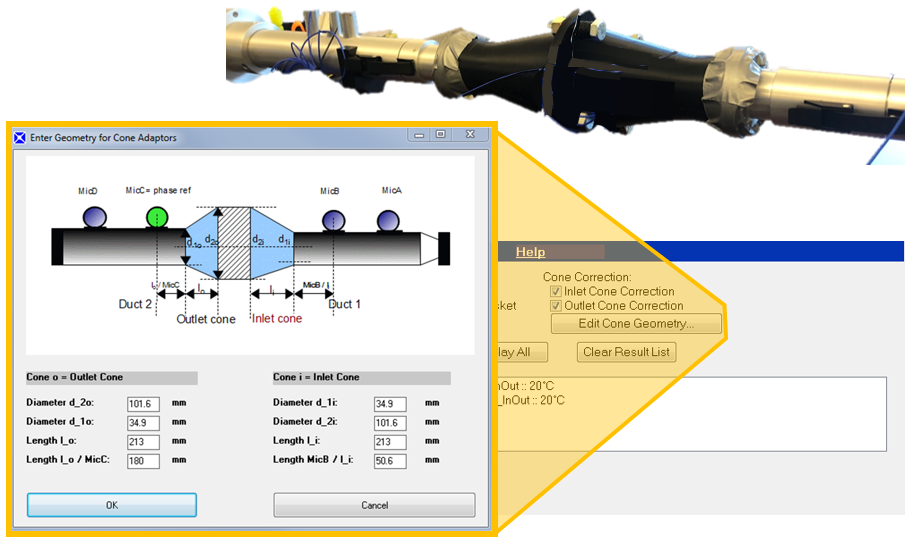
Figure 29: Cone correction menu in Simcenter Testlab.
The correction can be setup before or after the measurement:
-
Cone Geometry – First enter the cone geometry
-
Apply Correction – Check ON the Inlet and Outlet Cone Correction check box, and push “Process” and then display.
The results for the pictured set of cones is shown in Figure 30.
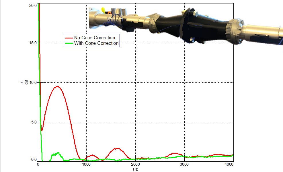
Figure 30: Sound transmission loss measurement of cones only uncorrected (red) and corrected (green).
Cone correction brings the Transmission Loss back to near zero dB.
In the result list, the cone correction used is annotated as shown in Figure 31.
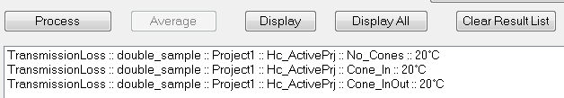
Figure 31: Results list in Transmission Loss.
The annotation includes:
- “No_Cones” when no cone correction is applied.
- “Cone_In” when correction is done only on the inlet.
- “Cone_InOut” when correction is performed on both the inlet and outlet.
- what about correction only done on the outlet?
In the active project, the data is organized as follows (Figure 32):
- Sound Transmission Loss (STL) results are automatically stored in a separate section called STL
- Hc contains the phase calibration (also in a separate section?)
- The acoustic FRFs used in the calculation of STL are stored in sections with the material name
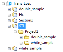
Figure 32: Results list in Testlab Navigation tree.
Hope these instructions measuring sound transmission loss where useful!
Questions? Email peter.schaldenbrand@siemens.com or contact Siemens Support Center.
Related Links: