Modal Testing: In structural testing, especially for Modal Testing, the quality of the Frequency Response Function (FRF) is very important. For correlation with an FE model, a good test modal model starts with a good, high fidelity FRF. The quality of the FRF is indicated in the Coherence function.
Typical Signals used for excitation: The types of excitation signals vary quite a bit, but are classified as either a random-stochastic type of signal, or one of sinusoidal nature. There are tradeoffs for both, and how they may be applied, but the signal-to-noise ratio (SNR) of the sinusoidal types is usually much better, resulting in a better FRF.
Avoid leakage in the Fourier Transform: A fundamental requirement for an accurate Fourier Transform is that the measured data sample is periodic within the acquisition window. Some signals are naturally periodic, like a burst-random, and some need to have a window to force the periodicity, which will always introduce some distortion in the measured data. For a sinusoid that lines up on the Fourier grid, this is a naturally periodic signal, and with high SNR.
Sine
- Naturally periodic at spectral lines
- Concentrate energy in spectral bands
- Hign SNR
Burst Random
- Naturally periodic
- Broad energy across frequencies
- Low SNR
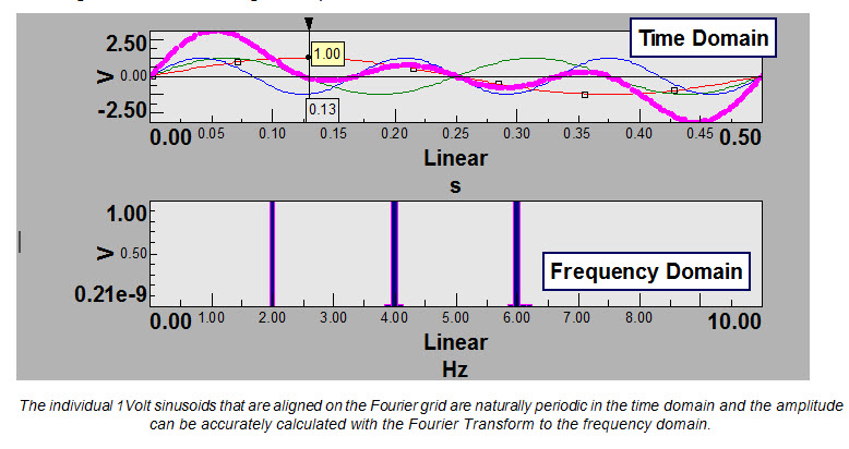
Multi-sines: Taking a number of these periodic sinusoids and adding them together are called “multi-sines”. Take for example a signal at 2, 4, and 6 Hertz, add them together, you end up with a signal as shown in the upper display below. With an acquisition window of .5 seconds, you end up with a frequency resolution on the Fourier grid of 2Hz, and so all signals are periodic.
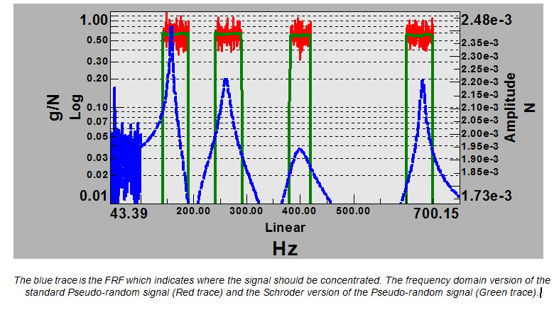
The picture below shows the difference of a Pseudo-random vs Broadband random and how they are represented in the frequency domain.

Different forms of “Multi-sines”: There are many combinations of “Multi-sines”, 2 of which are used for FRF excitation signals.
- Periodic Random - Random Amplitude Spectrum with Random Phase.
- Pseudo Random - Fixed Amplitude Spectrum with Random Phase. Can be a Constant Amplitude Spectrum or Shaped Amplitude Spectrum to concentrate energy around the resonances
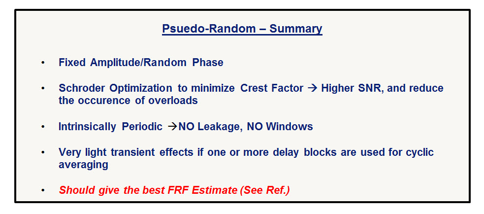
With the Pseudo-random signal, there is control on the amplitude to define the sinusoids used to excite the structure. The amplitudes can be shaped to correspond with higher amplitudes where the structural resonance occurs. This puts more of the shaker excitation energy where it is most needed. By manipulating the phases of the Pseudo-random signal with “Schroder” sines, this can reduce the crest factor, (the peak to RMS ratio) of the output voltage to the amplifier/shaker combination. This will keep the time and spectral excitation signals closer to the reference spectrum. The benefit of this can be seen in the green trace of the display. In this case you can raise the excitation level higher, but still avoiding overloads, which can ruin a measurement.
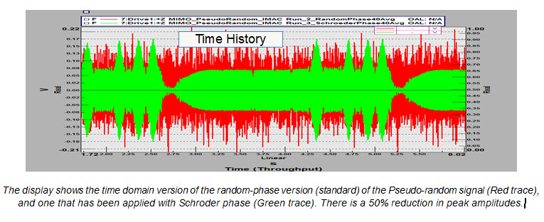
Play the videos to hear the difference between random phase and Schroder phase signals of the same reference spectrum:
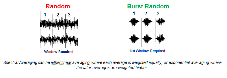
Spectral averaging: To measure a good representation of the signal, then a certain number of averages are required. The signal-to-noise has a big part in how many are required, and since sinusoidal signals have a better SNR, they will generally require less number of averages, saving testing time. For random data averaging in the frequency domain, there is a choice of linear or exponential averaging, whether using random with windowing, or more commonly using burst random.
Cyclic Averaging: A time domain version of averaging is called cyclic averaging. There are a couple of cases where this is done.
- Case 1: Semi-stationary conditions
- “Adaptive resampling”
- Sampling based on RPM, also called Order Tracking
- Case 2: Stationary conditions
- Synchronous sampling - Time average starts at beginning of time block or event

Cyclic averaging can be done when there is a repeated time signal exciting the structure, and the averaging is done “cyclically” in time, corresponding with the period of excitation. After some “delay blocks” have been sent, the transients have a chance to decay, and the structure has some time to respond periodically to that signal. The averaging is started after a number of these “Delay blocks”, and then repeated at the same time after each excitation signal. After a number of these so-called “inner-loop” averages, then a number of “outer-loop” averages are taken.
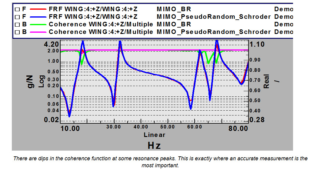
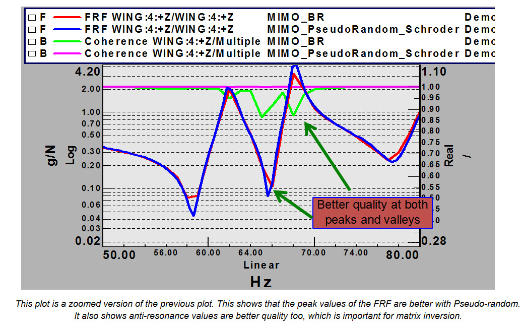
Case Studies: To show the benefit of this Pseudo-random technique on a real structure, the following data is shown for a set of “Driving-point” FRF’s made on an airplane. The following graphs use the Coherence function as a measure of the FRF quality. A value of 1.0 is a perfect coherence, and hence good quality FRF. You can see there are some lower dips in the coherence for the Burst Random case compared with the Pseudo-random with Schroder Sines case.
Reference: sem.org-IMAC-XIV-14th-Int-14-14-2-Cyclic-Averaging-Frequency-Response-Function-Estimation – Allemang, Phillips
Reference: sem.org-2011_IMAC_Advanced shaker excitation signals for aerospace testing – Peeters, Carrella, Lau, Gatto, Coppotelli
Questions? Post a reply or email chris.sensor@siemens.com.
Modal Data Acquisition:
Modal Analysis and Operational Deflection Shapes:


